Distributed Sampling on Dask Bags
Contributing to open-source projects is a rewarding experience. Even though the contribution regards a small amount of code, being aware that those few lines will be used by many users, many times, in the future, gives a really satisfying feeling.
The workflow was simple, I went on the issue tracker of the project, I selected a new feature to implement which I knew was not impossible to implement, then I manifested my intentions and I started working on it.
The challenging part of this work was to prove its mathematical correctness.
I had the initial idea since the beginning, but writing its proof helped me out to improve the algorithm and to fix its corner cases.
First I will introduce Dask and the concept of distributed data structure, then I will briefly describe the problem of sampling and my proposed solution, including a small proof of correctness and some words on its computational complexity. I will conclude with a statistical test to show that one generated result is not unbalanced.
Dask
Dask is a distributed framework to perform data analysis, if you know Apache Spark, you can easily understand what we’re talking about. Let’s say, Dask is an alternative to Apache Spark, but written in python and backed by Anaconda Inc. You can find here an interesting article describing the differences between the two. I won’t go into my feeling that the Dask project will become the next big thing in the data analysis world.
My first contribution was about a specific distributed data structure called: Bag. In Math terms a Bag is a Multiset, which can be thought of as a python list where the order of its elements is not meaningful; in other words, data are inserted following an order which is not necessarily the same when they are read.
Distributed Data Structure
Those data structures are not typical data structures studied on Algorithm classes at CS degrees. Those are distributed, which means they do not necessarily reside on the same machine. In other words, those data structures are usually divided into partitions that are stored in memory, possibly on different workers of the same cluster. A key point here is that all algorithms that operate over distributed data structures must take into account that data communications among different workers are time-consuming since they are dominated by network performances.
Sampling
The feature implemented is sampling, more specifically simple sampling, with or without replacement. I will not explain the definition of sampling or the difference between with or without replacement since online there are plenty of resources on it.
Interface
The philosophy of Dask is to minimize the efforts on readapting code written for non-distributed data structures, in the case of a Bag, its non-distributed python versions are lists or their abstraction: sequences.
I implemented a new method in the Bag class, I named it after python the random.choices function and I decided to follow closely its interface.
Here’s an example:
import randomseq = [1, 2, 3, 4, 5, 6]s = random.choices(seq, k=2)print(s)>> [2, 6]
Here’s the code using the newly implemented method:
import dask.bag as db
from dask.bag import randomseq = db.from_sequence([1, 2, 3, 4, 5, 6], npartitions=3)s = random.choices(seq, k=2)print(list(s.compute()))>> [2, 6]
Two steps algorithm
The proposed solution is implemented with map and reduce. It performs two sampling steps: one on maps and one on reduce. The first sampling is done over all the elements of every single partition, as a result, all elements drawn from the same partition are selected with the same equal probability.
By using this approach, elements belonging to different partitions are selected with different probability, since partitions do not necessarily have the same size.
To counterbalance this unfairness, when the sampled elements are gathered on the reduce, a weighted sampling is performed.
Weights used on the reduce are computed taking into account specific properties of the partition where each element comes from, like the number of elements of the partition or the real number of elements selected during the first sampling. Those properties are cleverly passed from the maps to reduce alongside the sampled elements.
After this initial description of the algorithm, now I will outline the math behind it.
Informal Proof
Here I will give informal proof on how a simple sampling is equivalent to two consequent weighted sampling procedures.
Let’s first assert the equivalence between simple sampling and weighted sampling with weights all equal to 1/N. This result will not be proven here.
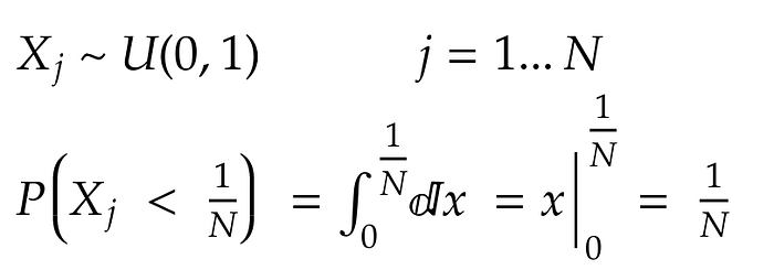
Since the procedure selects k random elements, on each selection and for each element j in the Bag: the probability to pick that element is 1/N.
Let’s rewrite the algorithm by associating to each element a random variable X with a uniform distribution between 0 and 1. The element is selected by the algorithm if X is smaller than the associated weight 1/N. In other words, an element is selected with probability equal to its weight.
In formulae:
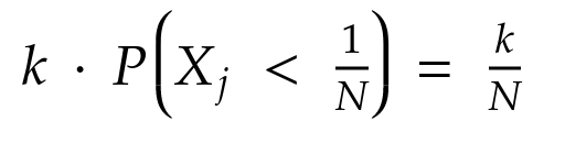
Since selections are made with replacement and probabilities of selection over k iterations are independent: the joint probability is the product of the probability of the single selections:
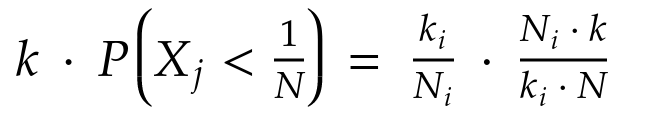
By leveraging the properties of the specific partition where the i-th element comes from, let’s rewrite it as the product of two ratios:

Here, k i-th is the actual number of elements extracted from the i-th partition, N i-th is the number of elements of that partition.
By substituting we obtain:
Now, let’s define two random variables F and S for each element in the Bag. The former is associated with the map phase and the latter with the reduce. Their distribution is uniform between 0 and 1:
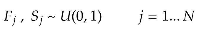
Where j is the associated element in the Bag.
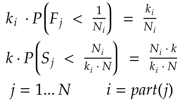
Now, by using the same procedure as before, let’s define two weighted sampling procedures based on those just defined random variables:

Where i is the partition associated with the element j.
By doing so, we obtain two weighted sampling procedures, where not all weights are equal to 1/N, but instead, each weight is specifically associated with an element and the partition where it belongs to.
Now, since we want to obtain the previous decomposition, the first sampling procedure must be repeatedly k i-th times and the second k times. Is important to stress out that k i-th and k can be different since the number of elements in each partition (N i-th) can be smaller than k. In those cases, the used k i-th is forced to be N i-th.
In formulae:
By substituting, we obtain:
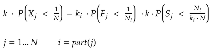
So, a simple sampling can be split into two distributed weighted sampling procedures and, by wisely choose the parameters of those procedures, is possible to keep unaltered the probability to select each element in the population.
Computational Costs
The proposed solution uses python random.choices both on maps and on reduce phases. So, its computational complexity is proportional to the original one. Regarding the amount of data passed from maps to the reduce, hence through the network, each map transfers k elements to the reduce. Given p the number of partitions: the number of sampled elements transferred on the network is O(k*p).
Which leads to be an acceptable behavior when k is small.
Statistical Test
To assess algorithm correctness here is performed a statistical test on a small example.
To test the correctness of the sampling procedure let’s compare it to a dice toss. In other words, the probability to sample one element is a random variable with a multinomial distribution with a parameter vector made by N elements all with value 1/N.
The idea here is to execute the experiment many times and count the occurrences of each element of the sequence. By doing so, we will expect all single occurrences to be close to their expected value, which is T/N, where T is the number of executions. The point is to leverage a statistical test that shows if the real performance of the experiment lays too far from the expected value.
The test sequence is made by 6 integers and two slightly unbalanced partitions: one partition is made by 4 elements and the other by 2.
The experiment involved 150 random selections of only one element.
Here’s the code:
import dask.bag as db
numbers = range(6)
buckets = {i: 0 for i in numbers}
a = db.from_sequence(numbers, partition_size=4)
for i in range(150):
    s = a.sample(k=1).compute()
    for e in s:
        buckets[e] += 1
print(buckets)
The expected value is 150/6=25.
We obtained the following occurrences of the six elements of the sequence:
25,26,33,22,17,27.
For this experiment I used R and XNomial package:
install.packages('XNomial')
require(XNomial)obs = c(25,26,33,22,17,27)
n = length(obs)
expr = rep(1/n, n)xmulti(obs, expr, statName = "LLR", histobins = T, histobounds = c(0, 0), showCurve = T)
Here’s a plot for the test log-likelihood ratio, which, under the null-hypothesis, asymptotically converges to a chi-squared distribution with 5 degrees of freedom:
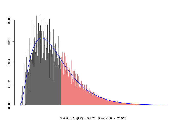
P value  (LLR)  =  0.3335
P value (Prob)  =  0.3339
P value (Chisq) =  0.3428
Obtaining as test outcome a p-value of 0.33.
By using a significance level α of 0.05, we cannot reject the null hypothesis that the distribution is multinomial with parameter vector 1/N.
More information about the theory behind this test is here, and the R package here.
Conclusions
In this article, I described a solution for the problem of distributed sampling.
As a further development, it will be interesting to investigate its use on other types of distributed data structures.
Additionally, by using Dask internal API, I figured out possible places of refactoring, especially between the HighLevelGraph and Bag classes, since there is not always a clear picture of the division of responsibilities among the two.
By the way, this is quite common on open source projects, since is not always easy for main contributors to plan the right balance between the types of tasks to assign. In other words, is not simple to drive free contributions among different task types, such as new features, bug fixing, or refactoring.
To keep track of the entire workflow here’s the link to the Github initial issue and my pull request.